Thermodynamic integration
Thermodynamic integration is a
general scheme to compute the free energy difference F - F0 between
two systems whose potential energies are U and U0 respectively.
The free energy difference F - F0 is the
reversible work done when the potential energy function U0 is
continuously and reversibly switched to U. To do this switching, a
continuously variable energy function  is defined such that
for
is defined such that
for
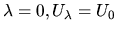 and for
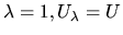 . We
also require to be differentiable with respect to
. We
also require to be differentiable with respect to
 for
for
 . A convenient form is:
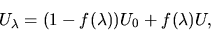 |
(1) |
where
 is an arbitrary continuous and differentiable
function of with the property f(0)=0 and f(1)=1. The
Helmholtz free energy of this hybrid system is:
is an arbitrary continuous and differentiable
function of with the property f(0)=0 and f(1)=1. The
Helmholtz free energy of this hybrid system is:
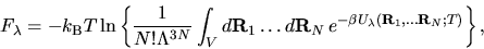 |
(2) |
Differentiating this with respect to gives:
 |
(3) |
so
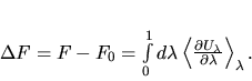 |
(4) |
A simple way of defining is:
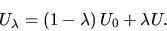 |
(5) |
Differentiating U with respect to and substituting
into Equation 4 yields:
with respect to and substituting
into Equation 4 yields:
 |
(6) |
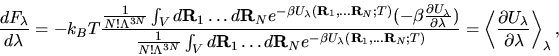
Under the ergodicity hypothesis, thermal averages are equivalent to time
averages, so we can calculate
 using molecular dynamics (MD), taking averages over time, with the evolution of the system
determined by the potential energy function .
It is important to stress that
the choice of the reference system does not affect the final answer
for F, although it does affect the efficiency of the calculations.
The latter can be understood by analysing the quantity
using molecular dynamics (MD), taking averages over time, with the evolution of the system
determined by the potential energy function .
It is important to stress that
the choice of the reference system does not affect the final answer
for F, although it does affect the efficiency of the calculations.
The latter can be understood by analysing the quantity
 . If this difference has large fluctuations then
one would need very long simulations to calculate the average value to
a sufficient statistical accuracy. Moreover, for an unwise choice of
U0 the quantity
may strongly
depend on so that one would need a large number of
calculations at different 's in order to compute the integral
in Eq. 6 with sufficient accuracy. It
is crucial, therefore, to find a good reference system, where "good"
means a system for which the fluctuations of U - U0 are as small as
possible. In fact, if the fluctuations are small enough, we can
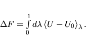
simply write
. If this difference has large fluctuations then
one would need very long simulations to calculate the average value to
a sufficient statistical accuracy. Moreover, for an unwise choice of
U0 the quantity
may strongly
depend on so that one would need a large number of
calculations at different 's in order to compute the integral
in Eq. 6 with sufficient accuracy. It
is crucial, therefore, to find a good reference system, where "good"
means a system for which the fluctuations of U - U0 are as small as
possible. In fact, if the fluctuations are small enough, we can
simply write
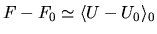 , with the
average taken in the reference ensemble. If this is not good enough,
the next approximation is readily shown to be:
, with the
average taken in the reference ensemble. If this is not good enough,
the next approximation is readily shown to be:
![\begin{displaymath}F - F_0 \simeq \langle U -
U_0 \rangle_0 - \frac{1}{2 k_{\rm...
...0 -
\langle U - U_0 \rangle_0
\right]^2 \right\rangle_0.
\end{displaymath}](img17.gif) |
(7) |
This form is particularly convenient since one only needs to sample
the phase space with the reference system.
In our case F is the free energy of the QMC system,
and F0 that of the DFT system, which acts as reference system.
Presumably, DFT is already a "good" reference system, in the sense defined
above, so that we will be able to use Eq. 7 for the
difference F - F0. The procedure will be to sample the phase space with
DFT-MD, and calculate QMC energies at a number of statistically independent
configurations extracted from the this simulation. This will be repeated for
both solid and liquid.
Dario Alfe`
2002-03-21